8.1 What are elliptic curves?

Historically, elliptic curves are rooted in so-called Diophantine equations, named after ancient Greek mathematician Diophantus of Alexandria. Diophantine equations are polynomial equations in two or more unknowns for which only integer solutions are of interest.

In the 19th century, these studies became more formalized and were extended to so called algebraic curves, which are the set of zeros of a polynomial of two variables in a plane. Circles, as defined as the zeros of

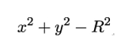
and ellipses, defined as the zeros of

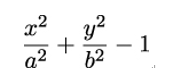
are the most common examples of algebraic curves. However, elliptic curves are not ellipses. They arose from the study of so-called elliptic integrals, by which the arc length of ellipses is computed, and were intensively studied by pure mathematicians in the 19th and early 20th century. They are characterized by their amazing property of possessing a way to add curve points, so that the result is another point on the curve.

In 1985, Victor Miller and Neil Koblitz independently proposed using elliptic curves in public-key cryptography. According to [102], these were the reasons:

• Greater flexibility, because there are many elliptic curves to choose from
• The absence of subexponential algorithms for finding discrete logarithms on suitably chosen curves

Our goal in this section is to define mathematically what we really mean by the term elliptic curve and to discuss some of their properties.

8.1.1 Reduced Weierstrass form

Our story starts with the set of zeros of a general cubic polynomial in two variables – x,y:

This is an example of an algebraic curve.

Obviously, we must be able to add and multiply the x,y and the coefficients together, therefore we require them to come from a field 𝔽, as defined in Chapter 7, Public-Key Cryptography. Through a series of coordinate transformations and after suitable re-naming of coefficients, we arrive at a much simpler equation, which is the defining equation for elliptic curves.

An elliptic curve E over a field 𝔽 is the set of points (x,y), where x,y and the coefficients ai are in 𝔽, satisfying the equation

along with some special point O at infinity.

This is called the Weierstrass form of E. We will explain a bit later what this ominous point O really is, but let’s start by looking at the defining equation. In the 19th century, mathematicians studied elliptic curves mostly over ℝ or ℂ, and real numbers are the best field to visualize an elliptic curve, as in Figure 8.1.

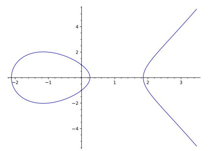
Figure 8.1: Elliptic Curve y2 = x3 − 4x + 1 over real numbers

Note the symmetry of the curve with respect to the x axis. This is because of the y2 on the left-hand side of the curve equation. We can make sure all elliptic curves have this symmetry by making another coordinate transformation. If we use

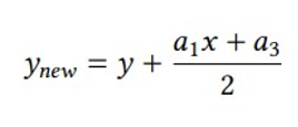
instead of y, we can get rid of the xy term on the left-hand side. A similar change, xnew = x + a2∕3, frees us from the x2 term on the right-hand side. After cleaning up and renaming the constants, we arrive at the reduced Weierstrass form of the elliptic curve,

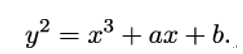
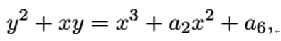
However, this only works if we are allowed to divide by 2 and by 3, i.e. if 2≠0 and 3≠0 in 𝔽. The fancy term for this requirement is the field characteristic should be larger than 3. If we work in a field 𝔽p, where p > 3, this is not a problem. But computers are especially efficient when dealing with bitstrings. Bitstrings live in the fields 𝔽2k, which do have characteristic 2. In this case, there are two possibilities for the reduced form:

• The nonsupersingular case

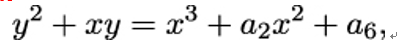
• The supersingular case

For example, the curve y2 + y = x3 over 𝔽⊭ is supersingular. As it turns out, supersingular curves are not as secure as nonsupersingular curves (see Section 8.4.2, Algorithms for solving special cases of ECDLP). Luckily, the vast majority of elliptic curves are nonsupersingular [102].